THUNDERMILL02 User Manual
This manual covers unpacking, connecting, installing and operating the THUNDERMILL02 electric field mill and its terminal unit.
Table of contents
Package Contents
- THUNDERMILL02 sensor unit (EFM) with Cat5e cable attached
- Terminal unit
- Power supply
The package contents may differ according to customer requirements.
Connection and Quick Functional Test
Connecting the System
The sensor communicates with the terminal over an cable with an RS485 interface.
- Connect the sensor to the terminal using the supplied cable.
- Connect the terminal to the power supply.
- The terminal starts automatically and the sensor begins to operate — the rotor starts spinning.
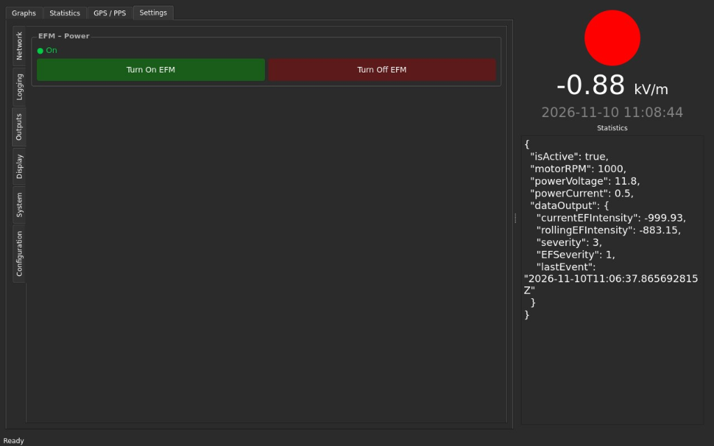
If the sensor rotor does not spin, open Settings → Outputs on the terminal and press Turn On EFM in the EFM – Power section. The indicator above the buttons shows the current state.
Quick Functional Test
With the system connected and the rotor spinning, bring an electrostatically charged object close to the sensing electrodes — for example a plastic bag rubbed against clothing. The electric field graph on the terminal home screen should react with a sharp change as the charge approaches and return back when it is moved away.
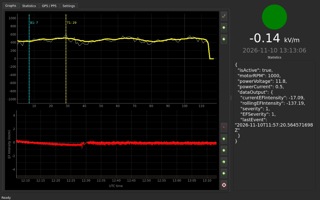
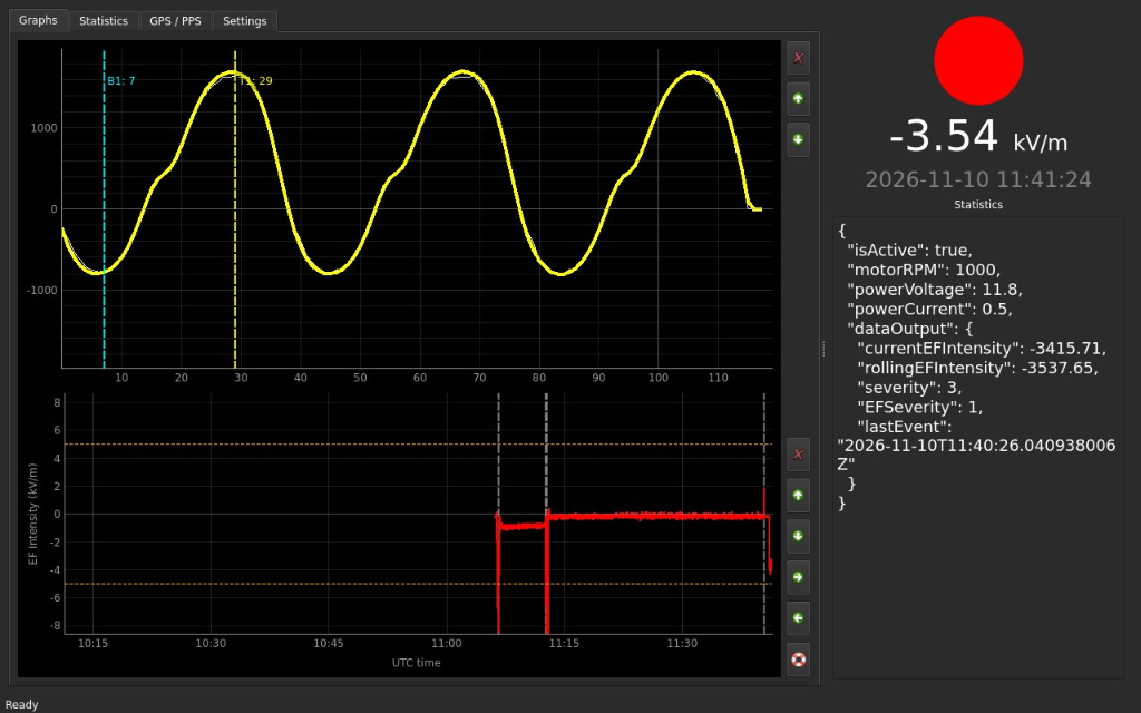
The upper graph on the home screen shows the raw signal from one rotor revolution, the lower graph shows the electric field intensity over time.
Without a charged object nearby, the raw signal is an almost flat line and the field intensity stays close to zero:
With a charged object near the sensor, the raw signal turns into a clear sine wave and the field intensity changes sharply:
Installation and Ideal Measurement Conditions
Install the sensor only in calm, clear weather with no thunderstorm expected. Keep the sensor, mast and all tools well away from overhead power lines — contact with a power line can be fatal. If you are not experienced with outdoor mast or antenna installation, have the installation done by a qualified installer.
Site Selection
The location of the sensor directly affects the measured values:
- Open area. Choose a place with a free view of the sky in all directions. Buildings, trees, poles and other tall objects nearby shield the sensor from the atmospheric field, so the readings will be too low. As a rule of thumb, apply the same siting rules as for an anemometer.
- Elevated position. In general, a higher and more exposed location gives better sensitivity. Keep in mind that any object raised above the surrounding ground (including the sensor itself and its mast) locally intensifies the electric field, so readings from an elevated sensor are higher than the undisturbed field — see Field Enhancement and Correction.
- Stable surroundings. Avoid locations where the geometry around the sensor changes (parked vehicles, growing vegetation, temporary structures), because every change of the surroundings changes the field enhancement.
- Easy access. The sensor needs little maintenance, but occasional cleaning or de-icing may be required. A location that can be reached easily and safely simplifies this.
Orientation
THUNDERMILL02 is mounted down-looking (sensing electrodes facing the ground) as standard. In this orientation, rain, snow, dust, insects and debris do not settle on the electrodes and their insulators, which keeps the measurement clean and reduces maintenance.

Mounting
The sensor is attached to the mount using the three nuts embedded in its bottom side. Make sure the mount is rigid — vibration and swaying of the mast are visible in the measured data.
Grounding
The sensor must be grounded, both for correct measurement and for lightning and electrical safety. Connect the sensor ground terminal and the metal mounting hardware to the central grounding point of the building (or to a dedicated ground rod in the field) using a suitably sized grounding conductor according to local electrical codes.
Weather Effects
Rain, snow and blowing dust carry electric charge. When charged particles hit the sensor, they appear as noise in the measured signal; during heavy precipitation this noise can be strong. It disappears once the precipitation stops.
Terminal Operation
Terminal Screens
The terminal application has four tabs: Graphs, Statistics, GPS / PPS and Settings. The panel on the right side is shown on all tabs:
- Indicator circle: the current warning level based on the field intensity (green = calm).
- Field intensity: the current electric field value in kV/m with the time (UTC).
- Statistics: the current value and the moving average of the field intensity (
currentEFIntensity,rollingEFIntensity), event severity, time of the last event, and the status of the sensor (motor speed, supply voltage and current).
Graphs
A conventional field mill shows the electric field intensity in kV/m. THUNDERMILL02 shows the complete signal measured during each rotor revolution (the waveform), from which this number is derived on top. You can therefore see not only what the sensor measures, but also how the value was obtained.
Upper graph — waveform. The signal from one rotor revolution, plotted against the sample number within the revolution.
- White line: waveform of the latest revolution.
- Yellow line: moving average of the waveform over the last revolutions. It suppresses noise and shows the stable shape of the signal.
- T1 and B1 markers: two sample positions in the revolution, where the sensing electrodes are fully exposed to the field (T1) and fully shielded (B1). The difference between the waveform values at these two points, multiplied by the calibration constant, gives the electric field intensity in kV/m.
The positions of T1 and B1 are set in Settings → Configuration using Find phase.
Lower graph — field intensity. The electric field intensity in kV/m over time (UTC), calculated from the T1 and B1 values of each revolution.
- Orange and red dashed lines: warning thresholds.
- Grey dashed lines: detected events (e.g. lightning discharges).
Because the full waveform is available, you can for example:
- see the effect of precipitation noise or interference directly in the signal;
- process the recorded raw waveforms with your own algorithms, independently of the terminal (see HDF5 File Content).
Statistics
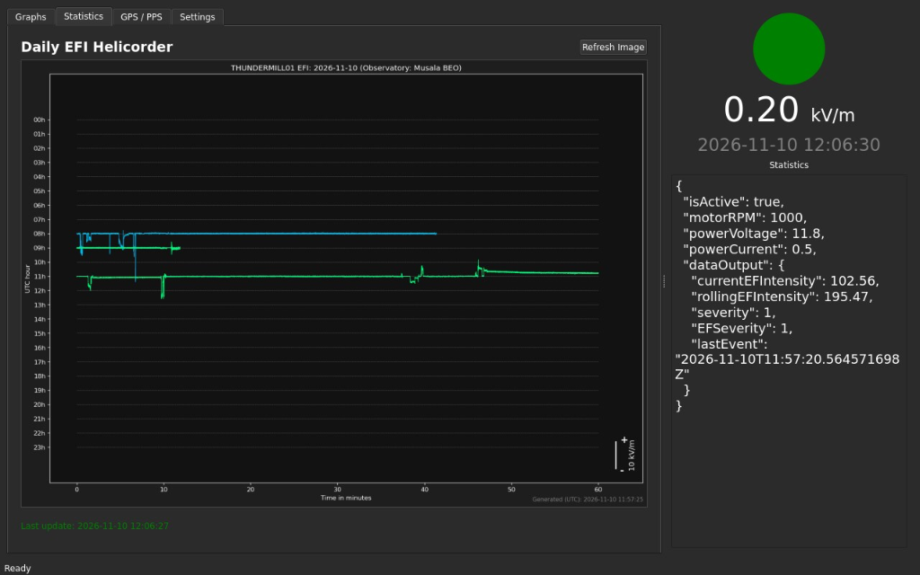
The Daily EFI Helicorder shows the electric field intensity of the current day — the same quantity as the lower graph on the Graphs tab, in a compact overview.
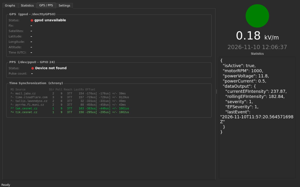
GPS / PPS
The terminal includes a GPS receiver for precise timing of all measured data. The tab shows:
- GPS: receiver status, fix, number of satellites, position and time.
- PPS: status of the pulse-per-second signal from the GPS receiver, used for precise time synchronization.
- Time Synchronization: sources used to synchronize the terminal clock (GPS/PPS and network time servers).
Settings
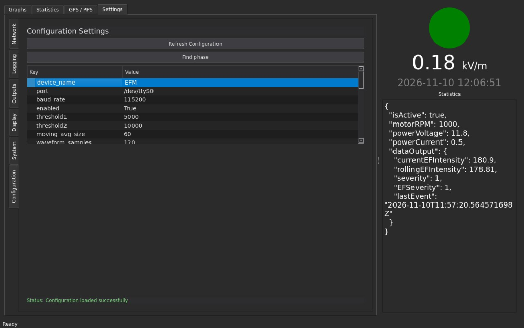
The Settings tab contains the configuration of the terminal and the sensor — network, data logging, outputs, display, system and measurement configuration.
Accessing the Terminal
The terminal can be operated directly on its touch display, or remotely over the network (Ethernet or Wi-Fi). The terminal is available on the network as mill.local:
- VNC — remote view and control of the terminal screen,
- SSH — remote command line, e.g.
ssh mill@mill.local.
Data Storage and Access
All measured data are stored on the internal SSD of the terminal in the /storage/EFM directory:
/storage/EFM/
├── waveform/
│   └── <YYYY>/<MM>/<DD>/
│       ├── <station>_<YYYYMMDD>_<HHMM>.h5
│       └── …
└── dayview/
    └── <YYYY>_<MM>/
        ├── <station>_EFI_HELICORDER_<YYYYMMDD>.png
        └── …
waveform/— measured data in HDF5 format. A new file is started every 10 minutes; the time in the file name is the start of the 10-minute interval. Data are written to the file in batches every 10 seconds.dayview/— daily helicorder images shown on the Statistics tab, one image per day.- All dates and times in directory and file names are in UTC.
<station>is the station name set in the terminal configuration.
HDF5 File Content
Each HDF5 file contains these datasets, one row per rotor revolution:
| Dataset | Type | Content |
|---|---|---|
waveform | int16, N × samples | Raw waveform of each revolution, zero-centred (raw ADC value − 32768) |
waveformmetadata | uint8, N × samples | Reserved |
metadata | compound, N | Timestamp and processed values of each revolution, see below |
Fields of the metadata dataset:
| Field | Description |
|---|---|
timestamp | Time of the revolution, milliseconds since 1970-01-01 UTC |
ef | Moving average of the field intensity, in raw units (multiply by the calibration constant ef_constant to get V/m) |
discharge | 1 if a discharge (e.g. lightning) was detected, otherwise 0 |
ef_channel_hi, ef_channel_low | Sample positions used to calculate the field intensity |
ef_phase_polarity | Field polarity set by Find phase (1 = positive, 2 = negative, 0 = not set) |
ef_top_channels, ef_bottom_channels | Sample positions shown as T and B markers in the waveform graph |
Example of reading a file in Python:
import h5py
import pandas as pd

with h5py.File("THUNDERMILL02_20261110_1140.h5", "r") as f:
    waveform = f["waveform"][:]           # shape (revolutions, samples)
    meta = pd.DataFrame(f["metadata"][:][["timestamp", "ef", "discharge"]])

meta["time"] = pd.to_datetime(meta["timestamp"], unit="ms", utc=True)
Downloading Data
The stored data can be downloaded over the network with rsync (or any other SSH-based tool, e.g. scp, WinSCP), using the credentials from Accessing the Terminal:
rsync -av mill@mill.local:/storage/EFM/ ./EFM/
Running the command repeatedly downloads only new or changed files.
FAQ
How to trigger an external device on an event (e.g. a camera)?
The terminal publishes detected events over the network as a WebSocket stream at:
ws://mill.local:8080/trigger
Any device on the same network can connect to it and react to the events. When the terminal detects a discharge (e.g. lightning), it sends a JSON message to all connected clients:
{"timestamp": "2026-11-10T11:40:26.040938006Z", "type": "TRIGG", "data": "Discharge_detected"}
The timestamp is in UTC. After an event, the next one is reported at the earliest after the decoupling period (discharge_decoupling_period in Settings → Configuration).
A minimal client in Python:
import asyncio, json, websockets

async def main():
    async with websockets.connect("ws://mill.local:8080/trigger") as ws:
        async for message in ws:
            event = json.loads(message)
            if event["type"] == "TRIGG":
                print("Event at", event["timestamp"])  # trigger your device here

asyncio.run(main())
Example: Lightning-Triggered Camera
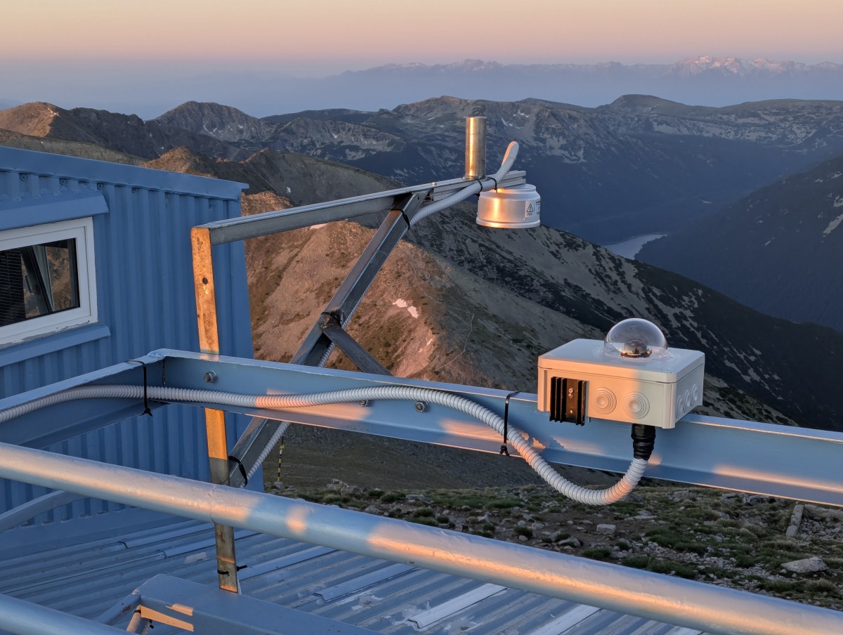
CircularPiCam is open-source software for a Raspberry Pi camera that records continuously into a ring buffer in memory. When a trigger arrives, it saves the frames from 2 seconds before and 2 seconds after the event, so the camera captures the whole lightning discharge, including its beginning.
To trigger the camera from THUNDERMILL02, run CircularPiCam with the WebSocket trigger pointing to the terminal:
python3 raw.py --websocket --websocket-url ws://mill.local:8080/trigger
With the --sync option, the captured frames can be automatically transferred over the network, for example to the terminal storage (--sync-dest mill@mill.local:/storage/CAM/). See the CircularPiCam documentation for installation and further options.
Can the sensor be used without the terminal?
Yes. The sensor sends its data as a plain ASCII stream over the RS485 interface, so it can be connected directly to a computer or a data logger. The stream format is described in THUNDERMILL02 Raw Data Format.
How to replace the cable?
The cable can be replaced, for example when a different cable length is needed.
Disconnect the terminal from the power supply before replacing the cable.
- Disassembly. Unscrew the three screws on the circumference of the sensor and pull the sensor body out of the housing.
- Connecting the new cable. Disconnect the cable from the sensor body and connect the new one.
- Reassembly. Insert the sensor body back into the housing and fasten the three screws.